-
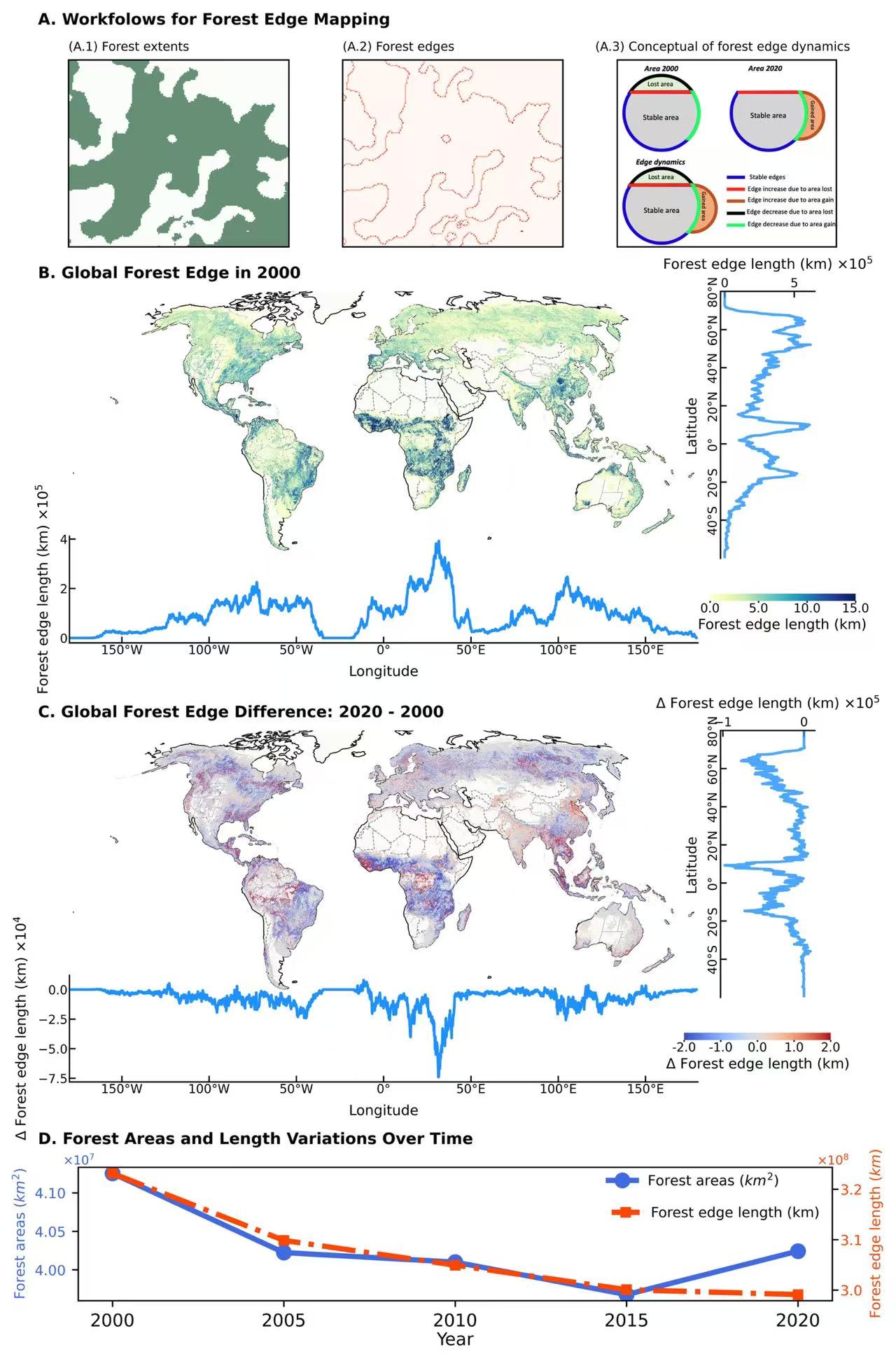
1. Global forest edge mapping
from osgeo import gdal
import numpy as np
import matplotlib.pyplot as plt
import cartopy.crs as ccrs
import cartopy.feature as cf
from scipy.ndimage import zoom
import matplotlib.ticker as mtick
import matplotlib as mpl
from cartopy.mpl.ticker import LatitudeFormatter, LongitudeFormatter
from mpl_toolkits.axes_grid1.inset_locator import inset_axes
import matplotlib.image as mpimg
import pandas as pd
import warnings
warnings.filterwarnings('ignore')
def read_data(image_data):
dataset = gdal.Open(image_data)
geotransform = dataset.GetGeoTransform()
origin_x,origin_y = geotransform[0],geotransform[3]
pixel_width, pixel_height = geotransform[1],geotransform[5]
width, height = dataset.RasterXSize, dataset.RasterYSize
lon = origin_x + pixel_width * np.arange(width)
lat = origin_y + pixel_height * np.arange(height)
data = dataset.GetRasterBand(1).ReadAsArray()
if data.max()>10000:
data = data/1000
data[data < 0.01] = np.nan
return data,lon,lat
def read_tif(tif_file):
dataset = gdal.Open(tif_file)
cols = dataset.RasterXSize
rows = dataset.RasterYSize
im_proj = (dataset.GetProjection())
im_Geotrans = (dataset.GetGeoTransform())
im_data = dataset.ReadAsArray(0, 0, cols, rows)
if im_data.ndim == 3:
im_data = np.moveaxis(dataset.ReadAsArray(0, 0, cols, rows), 0, -1)
dataset = None
return im_data, im_Geotrans, im_proj,rows, cols
def base_map(ax):
states_provinces = cf.NaturalEarthFeature(category='cultural',name='admin_1_states_provinces_lines',
scale='50m',facecolor='none')
ax.add_feature(cf.LAND,alpha=0.2)
ax.add_feature(cf.BORDERS, linestyle='--',lw=0.4, alpha=0.5)
ax.add_feature(cf.LAKES, alpha=0.5)
ax.add_feature(cf.COASTLINE,lw=0.5)
ax.add_feature(cf.RIVERS,lw=0.2)
ax.add_feature(states_provinces,lw=0.2,edgecolor='gray')
return
def lon_lat_stats(im_data, lon, lat):
lon_sum, lat_sum = np.nansum(im_data, axis = 0), np.nansum(im_data, axis = 1)
lon_sum = np.split(lon_sum, len(lon_sum)/10)
lon_sum = np.array([subarray.sum() for subarray in lon_sum])
lat_sum = np.split(lat_sum, len(lat_sum)/10)
lat_sum = np.array([subarray.sum() for subarray in lat_sum])
lat_statistical,lon_statistical = zoom(lat,0.1),zoom(lon,0.1)
return lat_statistical,lon_statistical, lat_sum, lon_sum
data1,lon,lat = read_data(f"/scratch/fji7/Forest_edge_mapping_2024_11_14/1_data/2000Edge.tif")
data2,lon,lat = read_data(f"/scratch/fji7/Forest_edge_mapping_2024_11_14/1_data/2020Edge.tif")
data = data2-data1
lat_statistical1,lon_statistical1, lat_sum1, lon_sum1 = lon_lat_stats(data1, lon, lat)
lat_statistical,lon_statistical, lat_sum, lon_sum = lon_lat_stats(data, lon, lat)
###
ex1,_,_,_,_ = read_tif(f"/scratch/fji7/Forest_edge_mapping_2024_11_14/1_data/Example_extent.tif")
ex2,_,_,_,_ = read_tif(f"/scratch/fji7/Forest_edge_mapping_2024_11_14/1_data/Example_edge.tif")
img = mpimg.imread('/scratch/fji7/Forest_edge_mapping_2024_11_14/1_data/conceptual_figure.png')
ex1 = ex1[50:200, 95:272]
ex2 = ex2[50:200, 95:272]
df = pd.read_csv("/scratch/fji7/Forest_edge_mapping_2024_11_14/1_data/Country_Forest_Area&Edge.csv")
years = [2000, 2005, 2010, 2015, 2020]
statis = df.sum(axis = 0)
areas = [statis[f"Total Forest Area {year} (KM2)"] for year in years]
edges = [statis[f"Total Forest Edge Length {year} (KM)"] for year in years]
years = [str(year) for year in years]
#************************************************************************************************************************************************************************************************
print("start plotting")
fig = plt.figure(figsize = (10,8))
config = {"font.family":'Helvetica'}
plt.subplots_adjust(hspace =0.3)
plt.rcParams.update(config)
# plot 2000 edge and 2020~2000 edge differences.
ax1 = fig.add_subplot(2,1,1,projection = ccrs.Robinson(central_longitude=0.0))
ax2 = fig.add_subplot(2,1,2,projection = ccrs.Robinson(central_longitude=0.0))
base_map(ax1)
base_map(ax2)
ax1.tick_params(axis='both',which='major',labelsize=8,direction='out',length=3,width=0.5,pad=1.3,labelleft = False, labelbottom = False,
bottom=False,left=False,top=False,right=False)
ax2.tick_params(axis='both',which='major',labelsize=8,direction='out',length=3,width=0.5,pad=1.3,labelleft = False, labelbottom = False,
bottom=False,left=False,top=False,right=False)
ax1.spines['geo'].set_linewidth(0)
ax2.spines['geo'].set_linewidth(0)
lons, lats = np.meshgrid(lon, lat)
### 2000 edges
cmap = 'YlGnBu'
max_value = 0
min_value = 15
lev = np.arange(0,15.1,5)
ax1.text(-0.05,1.05, f'B. Global Forest Edge in 2000', transform=ax1.transAxes, fontsize = 9,fontweight='bold')
ax1.set_extent([-179.99, 179.99, lat.min(), lat.max()])
p = ax1.pcolormesh(lons,lats,data1,transform=ccrs.PlateCarree(),cmap=cmap,vmin = min_value, vmax = max_value)
cax, kw = mpl.colorbar.make_axes(ax1, location='bottom', pad=0.06, shrink=0.15,anchor = (0.98,0.65))
cbar = plt.colorbar(p, cax=cax, orientation='horizontal',ticks=lev)
cbar.ax.xaxis.set_major_formatter(mtick.FormatStrFormatter('%.1f'))
cbar.outline.set_visible(False)
cbar.ax.tick_params(labelsize=7,pad = 0.1,length=1)
cbar.set_label('Forest edge length (km)',fontsize = 8,labelpad=2)
### 2000~ 2020 edges differences
cmap = 'coolwarm'
max_value = 2
min_value = -2
lev = np.arange(-2,2.1,1)
ax2.text(-0.05,1.05, f'C. Global Forest Edge Difference: 2020 - 2000 ', transform=ax2.transAxes, fontsize = 9,fontweight='bold')
ax2.set_extent([-179.99, 179.99, lat.min(), lat.max()])
p = ax2.pcolormesh(lons,lats,data,transform=ccrs.PlateCarree(),cmap=cmap,vmin = min_value, vmax = max_value)
cax, kw = mpl.colorbar.make_axes(ax2, location='bottom', pad=0.06, shrink=0.15,anchor = (0.95,0.65))
cbar = plt.colorbar(p, cax=cax, orientation='horizontal',ticks=lev)
cbar.ax.xaxis.set_major_formatter(mtick.FormatStrFormatter('%.1f'))
cbar.outline.set_visible(False)
cbar.ax.tick_params(labelsize=7,pad = 0.1,length=1)
cbar.set_label(r"$\Delta$ Forest edge length (km)",fontsize = 8,labelpad=2)
"""
***************************************************************************************************
"""
ax1_inset1 = inset_axes(ax1, width="100%", height="40%", loc='lower center', bbox_to_anchor=(0, -0.35, 1, 1),bbox_transform=ax1.transAxes)
ax1_inset2 = inset_axes(ax1, width="15%", height="100%", loc='center right', bbox_to_anchor=(0.2, 0, 1, 1),bbox_transform=ax1.transAxes)
###
ax1_inset1.plot(lon_statistical1, lon_sum1, c = 'dodgerblue', lw = 1.5)
ax1_inset1.set_xlim(lon.min(),lon.max())
ax1_inset1.xaxis.set_major_formatter(LongitudeFormatter())
ax1_inset1.set_facecolor('none')
ax1_inset1.tick_params(axis='both',which='major',labelsize=7,direction='in',pad=1,bottom=True, left=True,top=False,right=False)
ax1_inset1.spines[['top', 'right']].set_visible(False)
ax1_inset1.set_xlabel('Longitude',fontsize = 8,labelpad = 5)
ax1_inset1.set_ylabel(r"Forest edge length (km) $\times 10^5$",fontsize = 8,labelpad = 5)
ax1_inset1.ticklabel_format(style='scientific', scilimits=(0, 0), axis='y')
ax1_inset1.yaxis.offsetText.set_visible(False)
###
ax1_inset2.plot(lat_sum1,lat_statistical1, c = 'dodgerblue', alpha=0.8,lw = 1.5)
ax1_inset2.set_facecolor('none')
ax1_inset2.spines[['bottom', 'right']].set_visible(False)
ax1_inset2.tick_params(axis='both',which='major',labelsize=7,direction='in',labeltop=True,
labelbottom=False,pad=1,bottom=False, left=True,top=True,right=False)
ax1_inset2.xaxis.set_label_position('top')
ax1_inset2.set_ylim(lat.min(),lat.max())
ax1_inset2.set_xlabel(r"Forest edge length (km) $\times 10^5$",fontsize = 8,labelpad = 5)
ax1_inset2.set_ylabel('Latitude',fontsize = 8,labelpad = 5)
ax1_inset2.set_yticklabels([x.get_text() for x in ax1_inset2.get_yticklabels()],rotation=90, va='center')
ax1_inset2.yaxis.set_major_formatter(LatitudeFormatter())
ax1_inset2.ticklabel_format(style='scientific', scilimits=(0, 0), axis='x')
ax1_inset2.xaxis.offsetText.set_visible(False)
"""
***************************************************************************************************
"""
ax2_inset1 = inset_axes(ax2, width="100%", height="40%", loc='lower center', bbox_to_anchor=(0, -0.35, 1, 1),bbox_transform=ax2.transAxes)
ax2_inset2 = inset_axes(ax2, width="15%", height="100%", loc='center right', bbox_to_anchor=(0.2, 0, 1, 1),bbox_transform=ax2.transAxes)
###
ax2_inset1.plot(lon_statistical, lon_sum, c = 'dodgerblue', lw = 1.5)
ax2_inset1.set_xlim(lon.min(),lon.max())
ax2_inset1.xaxis.set_major_formatter(LongitudeFormatter())
ax2_inset1.set_facecolor('none')
ax2_inset1.tick_params(axis='both',which='major',labelsize=7,direction='in',pad=1,bottom=True, left=True,top=False,right=False)
ax2_inset1.spines[['top', 'right']].set_visible(False)
ax2_inset1.set_xlabel('Longitude',fontsize = 8,labelpad = 5)
ax2_inset1.set_ylabel(r"$\Delta$ Forest edge length (km) $\times 10^4$",fontsize = 8,labelpad = 5)
ax2_inset1.ticklabel_format(style='scientific', scilimits=(0, 0), axis='y')
ax2_inset1.yaxis.offsetText.set_visible(False)
###
ax2_inset2.plot(lat_sum,lat_statistical, c = 'dodgerblue', alpha=0.8,lw = 1.5)
ax2_inset2.set_facecolor('none')
ax2_inset2.spines[['bottom', 'right']].set_visible(False)
ax2_inset2.tick_params(axis='both',which='major',labelsize=7,direction='in',labeltop=True,
labelbottom=False,pad=1,bottom=False, left=True,top=True,right=False)
ax2_inset2.xaxis.set_label_position('top')
ax2_inset2.set_ylim(lat.min(),lat.max())
ax2_inset2.set_xlabel(r"$\Delta$ Forest edge length (km) $\times 10^5$",fontsize = 8,labelpad = 5)
ax2_inset2.set_ylabel('Latitude',fontsize = 8,labelpad = 5)
ax2_inset2.set_yticklabels([x.get_text() for x in ax2_inset2.get_yticklabels()],rotation=90, va='center')
ax2_inset2.yaxis.set_major_formatter(LatitudeFormatter())
ax2_inset2.ticklabel_format(style='scientific', scilimits=(0, 0), axis='x')
ax2_inset2.xaxis.offsetText.set_visible(False)
"""
***************************************************************************************************
"""
axx1 = inset_axes(ax1, width="60%", height="70%", loc='upper left', bbox_to_anchor=(-0.14, 0.9, 1, 1),bbox_transform=ax1.transAxes)
axx2 = inset_axes(ax1, width="60%", height="70%", loc='upper center', bbox_to_anchor=(0.11, 0.9, 1, 1),bbox_transform=ax1.transAxes)
axx3 = inset_axes(ax1, width="60%", height="70%", loc='upper right', bbox_to_anchor=(0.36, 0.9, 1, 1),bbox_transform=ax1.transAxes)
axx1.imshow(ex1, cmap = "Greens_r", alpha = 0.6)
axx2.imshow(ex2, cmap = "Reds", alpha = 0.8)
axx3.imshow(img)
axx1.tick_params(axis='both',which='both',bottom=False,left=False,labelbottom=False,labelleft=False)
axx2.tick_params(axis='both',which='both',bottom=False,left=False,labelbottom=False,labelleft=False)
axx3.tick_params(axis='both',which='both',bottom=False,left=False,labelbottom=False,labelleft=False)
ax1.text(-0.05,2, f'A. Workfolows for Forest Edge Mapping', transform=ax1.transAxes, fontsize = 9,fontweight='bold')
axx1.text(0,1.05, f'(A.1) Forest extents', transform=axx1.transAxes, fontsize = 7)
axx2.text(0,1.05, f'(A.2) Forest edges', transform=axx2.transAxes, fontsize = 7)
axx3.text(-0.1,1.05, f'(A.3) Conceptual of forest edge dynamics', transform=axx3.transAxes, fontsize = 7)
"""
***************************************************************************************************
"""
###
ax2.text(-0.05,-0.55, f'D. Forest Areas and Length Variations Over Time', transform=ax2.transAxes, fontsize = 9,fontweight='bold')
axx4 = inset_axes(ax2, width="120%", height="50%", loc='lower left', bbox_to_anchor=(0, -1.17, 1, 1),bbox_transform=ax2.transAxes)
axx4.plot(years, areas, color = "royalblue", marker = 'o',markersize=8,linewidth=3, label= r'Forest areas ($km^2$)')
axx4.set_xlabel('Year',fontsize = 10,labelpad = 1)
axx4.set_ylabel(r'Forest areas ($km^2$)', color='royalblue', fontsize = 8)
axx4.tick_params(axis='y', labelsize=8, labelcolor='royalblue')
axx4.ticklabel_format(style='scientific', scilimits=(0, 0), axis='y')
axx4.yaxis.offsetText.set_visible(False)
axx4.text(-0.02,1.02, r"$\times 10^7$", transform=axx4.transAxes, fontsize = 7, color = "royalblue")
axx4.legend(loc = 'upper right',fontsize=8, facecolor= 'none',edgecolor = 'none',bbox_to_anchor=(0.945, 1.05))
###
axx5 = inset_axes(ax2, width="120%", height="50%", loc='lower left', bbox_to_anchor=(0, -1.17, 1, 1),bbox_transform=ax2.transAxes)
axx5.set_facecolor('none')
axx5.plot(years, edges, color = "orangered", marker = 's',markersize=5,linewidth=3,ls = "-.", label='Forest edge length (km)')
axx5.set_ylabel(r'Forest edge length ($km$)', color='orangered', fontsize = 8)
axx5.tick_params(axis='y', labelcolor='royalblue')
axx5.spines[['top', 'left']].set_visible(False)
axx5.yaxis.set_label_position('right')
axx5.tick_params(axis='both',which='major',labelsize=8,direction='out',labeltop=False,labelright=True,labelleft=False,
labelbottom=False,pad=1,bottom=False, left=False,top=False,right=True)
axx5.tick_params(axis='y', labelcolor='orangered')
axx5.ticklabel_format(style='scientific', scilimits=(0, 0), axis='y')
axx5.yaxis.offsetText.set_visible(False)
axx5.text(0.98,1.02, r"$\times 10^8$", transform=axx5.transAxes, fontsize = 7, color = "orangered")
axx5.legend(loc = 'upper right',fontsize=8, facecolor= 'none',edgecolor = 'none',bbox_to_anchor=(1, 0.8))
plt.savefig('/scratch/fji7/Forest_edge_mapping_2024_11_14/2_exported_figures/Figure 1_Forest edge.png', dpi=1000, bbox_inches='tight')
-
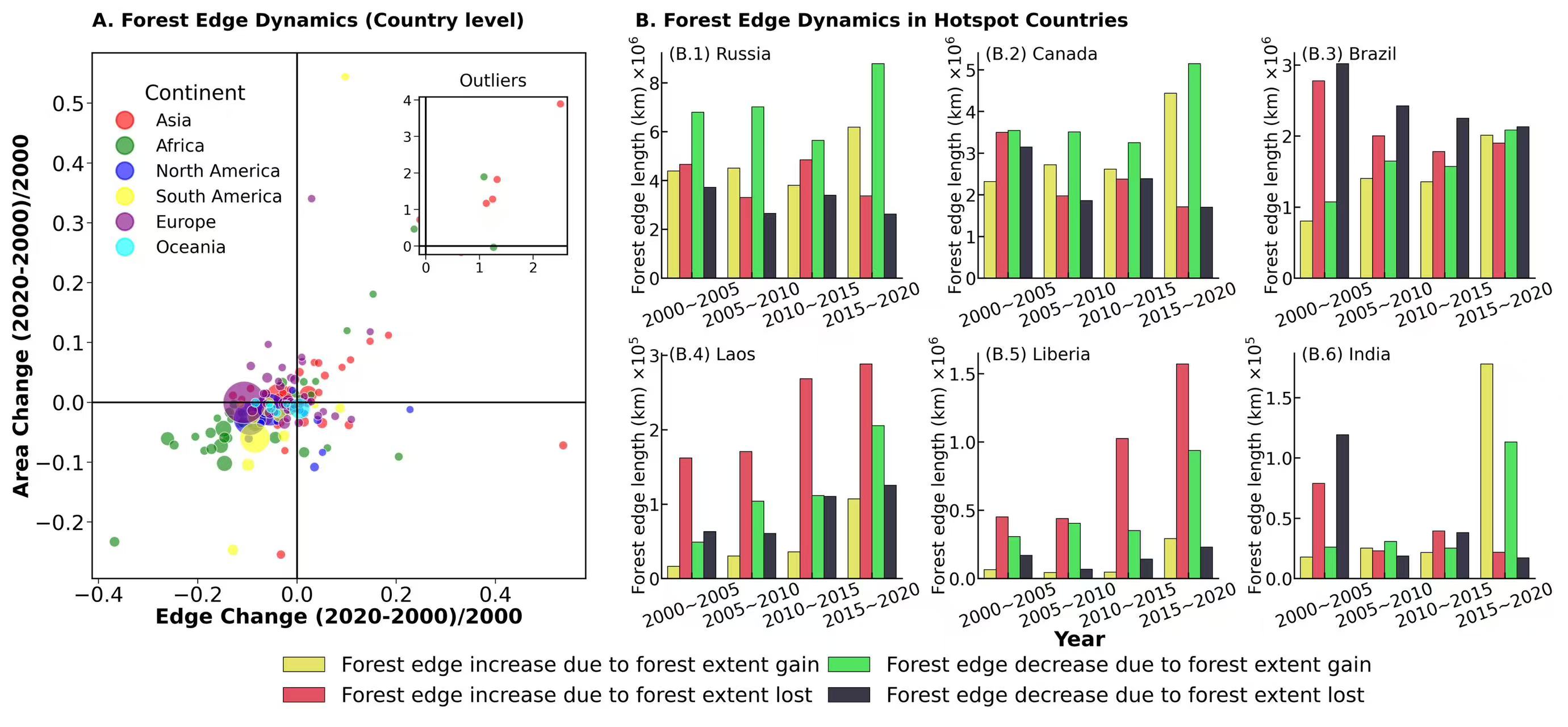
2. Global forest edge dynamics statistics
import matplotlib.pyplot as plt
import numpy as np
import pandas as pd
import seaborn as sns
from mpl_toolkits.axes_grid1.inset_locator import inset_axes
from matplotlib import gridspec
from matplotlib.lines import Line2D
import cartopy.io.shapereader as shpreader
import warnings
warnings.filterwarnings('ignore')
def custom_colormap(i, j, n):
# Normalize the indices to the range [0, 1]
x = i / (n - 1)
y = j / (n - 1)
# Compute the distance from the center
distance = np.sqrt((x - 0.5)**2 + (y - 0.5)**2)
# Define the color components based on distance from center
g = np.clip(distance + (x - 0.5), 0, 1)
r = np.clip(distance + (y - 0.5), 0, 1)
b = np.clip(1 - distance, 0, 1)
return (r, g, b, 1)
n = 40
bivariate_colors = np.empty((n, n, 4))
for i in range(n):
for j in range(n):
bivariate_colors[i, j] = custom_colormap(i, j, n)
#****************************************************************************************************************************************************************************************************************************************************
df = pd.read_csv("/scratch/fji7/Forest_edge_mapping_2024_11_14/1_data/processed_country_data_with_area.csv")
world_filepath = shpreader.natural_earth(resolution='10m', category='cultural', name='admin_0_countries')
reader = shpreader.Reader(world_filepath)
countries = [country.attributes['NAME'] for country in reader.records()]
continents = [country.attributes['CONTINENT'] for country in reader.records()]
country_to_continent = dict(zip(countries, continents))
df['continent'] = df['country'].map(country_to_continent)
colors = {'Asia': 'red','Africa': 'green','North America': 'blue','South America': 'yellow','Europe': 'purple','Oceania': 'cyan'}
df['Edge Change'] = df['Edge Change'].astype(float)
df['Area Change'] = df['Area Change'].astype(float)
df = df.dropna(subset=['Edge Change', 'Area Change'])
edge_change_threshold = 3 * df['Edge Change'].std()
area_change_threshold = 3 * df['Area Change'].std()
subset_df = df[(abs(df['Edge Change']) <= edge_change_threshold)& (abs(df['Area Change']) <= area_change_threshold)]
#****************************************************************************************************************************************************************************************************************************************************
selected_countries = ["Russia", "Canada", "Brazil", "Laos", "Liberia", "India"]
years = [2000, 2005, 2010, 2015, 2020]
start_var = True
for year in years[:-1]:
data = pd.read_csv(f"/scratch/fji7/Forest_edge_mapping_2024_11_14/1_data/country_data_with_area_{year}_{year+5}.csv")
data = data[data['Country'].isin(selected_countries)]
data = data[["Country", "Increase Increase Edge Length (KM)", "Increase Decrease Edge Length (KM)",
"Decrease Increase Edge Length (KM)", "Decrease Decrease Edge Length (KM)"]]
data["time_period"] = f"{year}~{year+5}"
if start_var:
final_data = data
start_var = False
else:
final_data = pd.concat([final_data, data], axis = 0)
final_data.reset_index(drop = True, inplace = True)
length_type = ["Increase Increase Edge Length (KM)", "Increase Decrease Edge Length (KM)",
"Decrease Increase Edge Length (KM)", "Decrease Decrease Edge Length (KM)"]
len_type = {"Increase Increase Edge Length (KM)":'Forest edge increase due to forest extent gain',
"Increase Decrease Edge Length (KM)":'Forest edge increase due to forest extent lost',
"Decrease Increase Edge Length (KM)":'Forest edge decrease due to forest extent gain',
"Decrease Decrease Edge Length (KM)":'Forest edge decrease due to forest extent lost'}
var = True
for length in length_type:
temp = final_data[["Country", "time_period", length]]
temp.rename(columns={length:'length'},inplace = True)
temp["len_type"] = len_type[length]
if var:
final_df = temp
var = False
else:
final_df = pd.concat([final_df, temp], axis = 0)
final_df.reset_index(drop = True, inplace = True)
#****************************************************************************************************************************************************************************************************************************************************
fig = plt.figure(figsize = (15,5.5))
gs = gridspec.GridSpec(21, 23)
config = {"font.family":'Helvetica'}
plt.subplots_adjust(hspace =0,wspace =0.25)
plt.rcParams.update(config)
ax = plt.subplot(gs[:, 0:8])
ax1 = plt.subplot(gs[0:9, 9:13])
ax2 = plt.subplot(gs[0:9, 14:18])
ax3 = plt.subplot(gs[0:9, 19:23])
ax4 = plt.subplot(gs[12:, 9:13])
ax5 = plt.subplot(gs[12:, 14:18])
ax6 = plt.subplot(gs[12:, 19:23])
#********
min_size = 20
max_size = 600
min_area = df['forest edge 2000'].min()
max_area = df['forest edge 2000'].max()
bubble_sizes = ((df['forest edge 2000'] - min_area) / (max_area - min_area) * (max_size - min_size) + min_size)
for continent, color in colors.items():
subset = subset_df[subset_df['continent'] == continent]
subset_bubble_sizes = bubble_sizes[subset.index]
ax.scatter(subset['Edge Change'], subset['Area Change'], s=subset_bubble_sizes, color=color, alpha=0.6, edgecolors="w", linewidth=0.5)
ax.scatter([], [], s=150, color=color, label=continent, alpha=0.6, edgecolors="w", linewidth=0.5)
ax.text(0,1.05, 'A. Forest Edge Dynamics (Country level)', transform=ax.transAxes, fontsize = 11,fontweight='bold')
ax.tick_params(axis='both',which='major',labelsize=12,direction='out',length=3,width=0.5,pad=1.3,labelleft = True, labelbottom = True,
bottom=True,left=True,top=False,right=False)
ax.set_xlabel('Edge Change (2020-2000)/2000',fontsize=12,labelpad = 1, fontweight='bold')
ax.set_ylabel('Area Change (2020-2000)/2000',fontsize=12,labelpad = 1, fontweight='bold')
legend = ax.legend()
handles = legend.legendHandles
labels = [text.get_text() for text in legend.get_texts()]
original_colors = [handle.get_facecolor() for handle in handles]
new_handles = [Line2D([0], [0], marker='o', label=label, color=color, markersize=10, linestyle='None') for label, color in zip(labels, original_colors)]
legend.remove()
ax.legend(handles=new_handles, labels=labels, title='Continent', bbox_to_anchor=(0, 0.97),
title_fontsize='large', loc='upper left', fontsize=10, facecolor='none', edgecolor='none')
ax.axvline(0, color='black', linestyle='-', linewidth=1) # x=0 line
ax.axhline(0, color='black', linestyle='-', linewidth=1) # y=0 line
axes = inset_axes(ax, width="30%", height="30%", loc='lower right', bbox_to_anchor=(-0.02, 0.6, 1, 1),bbox_transform=ax.transAxes)
for continent, color in colors.items():
outliers = df[(abs(df['Edge Change']) > edge_change_threshold)
| (abs(df['Area Change']) > area_change_threshold)]
subset = outliers[outliers['continent'] == continent]
subset_bubble_sizes = bubble_sizes[subset.index]
axes .scatter(subset['Edge Change'], subset['Area Change'], s=subset_bubble_sizes, color=color, alpha=0.6, edgecolors="w", linewidth=0.5)
axes.set_title('Outliers',fontsize = 10)
axes.axvline(0, color='black', linestyle='-', linewidth=1)
axes.axhline(0, color='black', linestyle='-', linewidth=1)
axes.tick_params(axis='both',which='major',labelsize=8,direction='out',length=3,width=0.5,pad=1.3,labelleft = True, labelbottom = True,
bottom=True,left=True,top=False,right=False)
#**********
ax.text(1.1,1.05, 'B. Forest Edge Dynamics in Hotspot Countries', transform=ax.transAxes, fontsize = 11,fontweight='bold')
axes = [ax1, ax2, ax3, ax4, ax5, ax6]
for i, axe in enumerate(axes):
temp = final_df[final_df["Country"]==selected_countries[i]]
sns.barplot(x='time_period', y= "length", hue = 'len_type', ax = axe, data=temp, palette=[bivariate_colors[n-1][n-1],bivariate_colors[0][n-1], bivariate_colors[n-1][0], bivariate_colors[0][0]],
saturation=0.7, errcolor='k',errwidth = 0.7,capsize = 0.07,edgecolor="k",linewidth = 0.4)
axe.legend(loc = 'lower right',fontsize=12,facecolor= 'none',edgecolor = 'none',bbox_to_anchor=(0.4, -0.65), ncol = 2,columnspacing = 0.4)
axe.ticklabel_format(style='scientific', scilimits=(0, 0), axis='y')
axe.yaxis.offsetText.set_visible(False)
for tick in axe.get_xticklabels():
tick.set_rotation(20)
axe.set_xlabel('')
expo = [6,6,6,5,6,5]
axe.set_ylabel(f"Forest edge length (km) $\\times 10^{{{expo[i]}}}$", labelpad = 0.1, fontsize = 10)
axe.spines[['top', 'right']].set_visible(False)
axe.tick_params(axis='both',which='major',labelsize=10,direction='in',labeltop=False,
labelbottom=True,pad=1,bottom=True, left=True,top=False,right=False)
axe.text(0.03,0.97, f'(B.{i+1}) {selected_countries[i]}', transform=axe.transAxes, fontsize = 10)
if i !=5:
axe.legend_.remove()
else:
axe.text(-1, -0.3, "Year", transform=axe.transAxes, fontsize = 12,fontweight='bold')
plt.savefig('/scratch/fji7/Forest_edge_mapping_2024_11_14/2_exported_figures/Figure 2_Forest edge dynamics statistics.png', dpi=600, bbox_inches='tight')
-
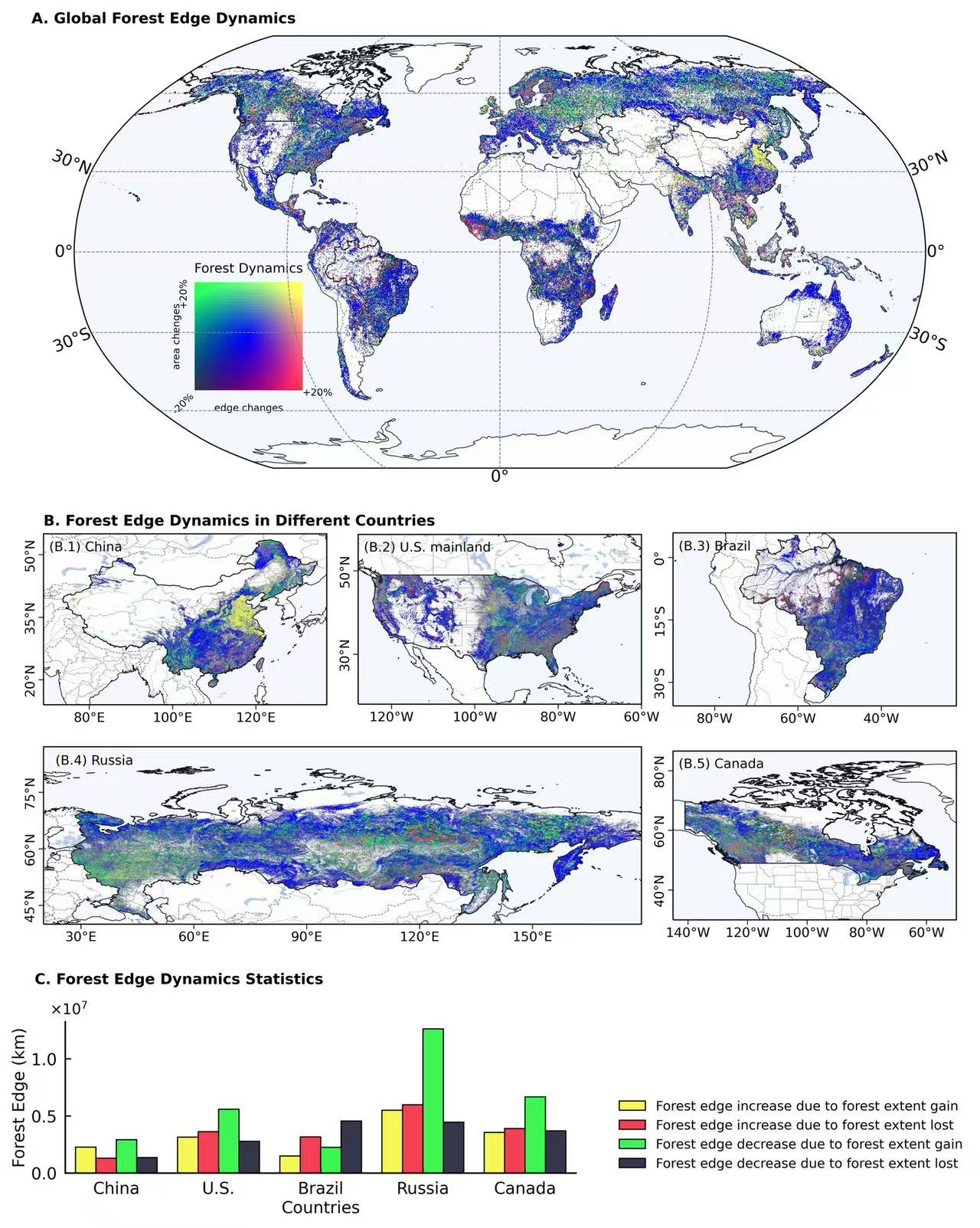
3. Global forest edge dynamiscs
import matplotlib.pyplot as plt
from osgeo import gdal
import numpy as np
import pandas as pd
import warnings
import seaborn as sns
from tqdm import tqdm
import cartopy.crs as ccrs
import cartopy.feature as cf
from cartopy.mpl.ticker import LatitudeFormatter, LongitudeFormatter
from mpl_toolkits.axes_grid1.inset_locator import inset_axes
import datetime
import geopandas as gpd
import xarray as xr
from shapely.geometry import mapping
from matplotlib import gridspec
import cartopy.io.shapereader as shpreader
warnings.filterwarnings('ignore')
def read_data(image_data):
dataset = gdal.Open(image_data)
geotransform = dataset.GetGeoTransform()
origin_x,origin_y = geotransform[0],geotransform[3]
pixel_width, pixel_height = geotransform[1],geotransform[5]
width, height = dataset.RasterXSize, dataset.RasterYSize
lon = origin_x + pixel_width * np.arange(width)
lat = origin_y + pixel_height * np.arange(height)
data = dataset.GetRasterBand(1).ReadAsArray()
dataset = None
return data,lon,lat,geotransform
def custom_colormap(i, j, n):
# Normalize the indices to the range [0, 1]
x = i / (n - 1)
y = j / (n - 1)
# Compute the distance from the center
distance = np.sqrt((x - 0.5)**2 + (y - 0.5)**2)
# Define the color components based on distance from center
g = np.clip(distance + (x - 0.5), 0, 1)
r = np.clip(distance + (y - 0.5), 0, 1)
b = np.clip(1 - distance, 0, 1)
return (r, g, b, 1)
def country_extraction(global_data,lat,lon,country_shp):
file = xr.DataArray(global_data, coords=[('lat', lat), ('lon', lon), ('channel', [1, 2, 3, 4])])
ds = xr.Dataset({'data': file})
ds.rio.write_crs("EPSG:4326", inplace=True)
ds = ds.rename({'lon': 'x'})
ds = ds.rename({'lat': 'y'})
clipped = ds.rio.clip(country_shp.geometry.apply(mapping), country_shp.crs, drop=False)
region_data = clipped.variables['data']
return region_data
def base_map(ax):
states_provinces = cf.NaturalEarthFeature(category='cultural',name='admin_1_states_provinces_lines',
scale='50m',facecolor='none')
ax.add_feature(cf.LAND,alpha=0.1)
ax.add_feature(cf.BORDERS, linestyle='--',lw=0.4, alpha=0.5)
ax.add_feature(cf.LAKES, alpha=0.5)
ax.add_feature(cf.OCEAN,alpha=0.1,zorder = 2)
ax.add_feature(cf.COASTLINE,lw=0.4)
ax.add_feature(cf.RIVERS,lw=0.2)
ax.add_feature(states_provinces,lw=0.2,edgecolor='gray')
return
#**********************************************************************************************
edge_file = '/scratch/fji7/Forest_edge_mapping_2024_11_14/1_data/2000_2020_edge_diff_per_range.tif'
area_file = '/scratch/fji7/Forest_edge_mapping_2024_11_14/1_data/2000_2020_area_diff_per_range.tif'
data1,lon1,lat1,transform1 = read_data(edge_file)
data2,lon2,lat2,transform2 = read_data(area_file)
mask = (data1>= -1) & (data1 <= 1) & (data2 >= -1) & (data2 <= 1)
data1[data1 < -1] = -1
data2[data2 < -1] = -1
data1[data1 > 1] = 1
data2[data2 > 1] = 1
print(np.nanmax(data1))
print(np.nanmin(data1))
print(np.nanmax(data2))
print(np.nanmin(data2))
data1_clipped = np.clip(data1, -0.2, 0.2)
data2_clipped = np.clip(data2, -0.2, 0.2)
data1 = None
data2 = None
data1_clipped_norm = (data1_clipped+0.2)/0.4
data2_clipped_norm = (data2_clipped+0.2)/0.4
data1_clipped = None
data2_clipped = None
print(np.nanmax(data1_clipped_norm))
print(np.nanmin(data1_clipped_norm))
print(np.nanmax(data2_clipped_norm))
print(np.nanmin(data2_clipped_norm))
n = 40
edge_indices = (data1_clipped_norm * (n - 1)).astype(int)
area_indices = (data2_clipped_norm * (n - 1)).astype(int)
bivariate_colors = np.empty((n, n, 4))
for i in range(n):
for j in range(n):
bivariate_colors[i, j] = custom_colormap(i, j, n)
final_rgba = np.zeros((*data1_clipped_norm.shape, 4))
for x in tqdm(range(final_rgba.shape[0])):
for y in range(final_rgba.shape[1]):
if mask[x, y]:
i = area_indices[x, y]
j = edge_indices[x, y]
final_rgba[x, y] = bivariate_colors[i, j]
else:
final_rgba[x, y] = [0,0,0,0]
world_filepath = shpreader.natural_earth(resolution='10m', category='cultural', name='admin_0_countries')
world = gpd.read_file(world_filepath)
countries = ['United States of America','China', 'Taiwan','Russia','Brazil','Canada']
selected_countries = world[world['SOVEREIGNT'].isin(countries)]
china = selected_countries[(selected_countries['SOVEREIGNT']=='China')|(selected_countries['SOVEREIGNT']=='Taiwan')]
us = selected_countries[(selected_countries['SOVEREIGNT']=='United States of America')&(selected_countries['TYPE']=='Country')]
russia = selected_countries[selected_countries['SOVEREIGNT']=='Russia']
brazil = selected_countries[selected_countries['SOVEREIGNT']=='Brazil']
canada = selected_countries[selected_countries['SOVEREIGNT']=='Canada']
contries_shp = [china, us, russia, brazil, canada]
start_t = datetime.datetime.now()
print('start:', start_t)
fig = plt.figure(figsize = (10,10))
gs = gridspec.GridSpec(21, 6)
config = {"font.family":'Helvetica'}
plt.subplots_adjust(hspace =0,wspace =0.25)
plt.rcParams.update(config)
####################### global data
ax = plt.subplot(gs[0:10, :],projection = ccrs.Robinson(central_longitude=0.0))
base_map(ax)
grd = ax.gridlines(draw_labels=True, xlocs=range(-180, 181, 90), ylocs=range(-60, 61, 30), color='gray',linestyle='--', linewidth=0.5, zorder=7)
grd.top_labels = False
ax.tick_params(axis='both',which='major',labelsize=8,direction='out',length=3,width=0.5,pad=1.3,labelleft = True, labelbottom = True,
bottom=True,left=True,top=False,right=False)
ax.spines['geo'].set_linewidth(0.7)
ax.text(-0.05,1.03, 'A. Global Forest Edge Dynamics', transform=ax.transAxes, fontsize = 9,fontweight='bold')
ax.imshow(final_rgba, extent = [lon1.min(), lon1.max(), lat1.min(), lat1.max()],transform=ccrs.PlateCarree(),zorder = 3)
china.plot(ax = ax,transform=ccrs.PlateCarree(),color = 'none',edgecolor="k",lw = 0.5)
us.plot(ax = ax,transform=ccrs.PlateCarree(),color = 'none',edgecolor="k",lw = 0.5)
russia.plot(ax = ax,transform=ccrs.PlateCarree(),color = 'none',edgecolor="k",lw = 0.5)
brazil.plot(ax = ax,transform=ccrs.PlateCarree(),color = 'none',edgecolor="k",lw = 0.5)
canada.plot(ax = ax,transform=ccrs.PlateCarree(),color = 'none',edgecolor="k",lw = 0.5)
axx = ax.inset_axes([0.08,0.18,0.25,0.25])
axx.set_aspect('equal', adjustable='box')
axx.imshow(bivariate_colors, origin='lower', extent=[0, 1, 0, 1])
axx.tick_params(axis='both',which='major',bottom=False, left=False,top=False,right=False,labelleft = False, labelbottom = False)
axx.spines[['top', 'right','left','bottom']].set_visible(False)
axx.set_title('Forest Dynamics',fontsize = 8)
axx.set_xlabel('edge changes',fontsize = 6,labelpad = 8)
axx.set_ylabel('area chenges',fontsize = 6,labelpad = 8)
axx.text(1,-0.05, '+20%', transform=axx.transAxes, fontsize = 6)
axx.text(-0.15,0.78, '+20%', transform=axx.transAxes, fontsize = 6,rotation= 90)
axx.text(-0.22,-0.22, '-20%', transform=axx.transAxes, fontsize = 6,rotation= 45)
####################### regional data
ax1 = plt.subplot(gs[11:16, 0:2],projection = ccrs.PlateCarree())
ax2 = plt.subplot(gs[11:16, 2:4],projection = ccrs.PlateCarree())
ax4 = plt.subplot(gs[11:16, 4:6],projection = ccrs.PlateCarree())
ax3 = plt.subplot(gs[16:21, 0:4],projection = ccrs.PlateCarree())
ax5 = plt.subplot(gs[16:21, 4:6],projection = ccrs.PlateCarree())
ax1.text(0,1.05, 'B. Forest Edge Dynamics in Different Countries', transform=ax1.transAxes, fontsize = 9,fontweight='bold')
ax1.text(0.02,0.9, '(B.1) China', transform=ax1.transAxes, fontsize = 8)
ax2.text(0.02,0.9, '(B.2) U.S. mainland', transform=ax2.transAxes, fontsize = 8)
ax4.text(0.02,0.9, '(B.3) Brazil', transform=ax4.transAxes, fontsize = 8)
ax3.text(0.02,0.9, '(B.4) Russia', transform=ax3.transAxes, fontsize = 8)
ax5.text(0.02,0.9, '(B.5) Canada', transform=ax5.transAxes, fontsize = 8)
d1 = country_extraction(final_rgba,lat1,lon1,china)
d2 = country_extraction(final_rgba,lat1,lon1,us)
d3 = country_extraction(final_rgba,lat1,lon1,russia)
d4 = country_extraction(final_rgba,lat1,lon1,brazil)
d5 = country_extraction(final_rgba,lat1,lon1,canada)
base_map(ax1)
base_map(ax2)
base_map(ax3)
base_map(ax4)
base_map(ax5)
ax1.imshow(d1, extent = [lon1.min(), lon1.max(), lat1.min(), lat1.max()],transform=ccrs.PlateCarree(), zorder = 3)
ax2.imshow(d2, extent = [lon1.min(), lon1.max(), lat1.min(), lat1.max()],transform=ccrs.PlateCarree(), zorder = 3)
ax3.imshow(d3, extent = [lon1.min(), lon1.max(), lat1.min(), lat1.max()],transform=ccrs.PlateCarree(), zorder = 3)
ax4.imshow(d4, extent = [lon1.min(), lon1.max(), lat1.min(), lat1.max()],transform=ccrs.PlateCarree(), zorder = 3)
ax5.imshow(d5, extent = [lon1.min(), lon1.max(), lat1.min(), lat1.max()],transform=ccrs.PlateCarree(), zorder = 3)
china.plot(ax = ax1,transform=ccrs.PlateCarree(),color = 'none',edgecolor="k",lw = 0.5)
us.plot(ax = ax2,transform=ccrs.PlateCarree(),color = 'none',edgecolor="k",lw = 0.5)
russia.plot(ax = ax3,transform=ccrs.PlateCarree(),color = 'none',edgecolor="k",lw = 0.5)
brazil.plot(ax = ax4,transform=ccrs.PlateCarree(),color = 'none',edgecolor="k",lw = 0.5)
canada.plot(ax = ax5,transform=ccrs.PlateCarree(),color = 'none',edgecolor="k",lw = 0.5)
ax1.set_extent([69, 137, 14, 50])
ax2.set_extent([-128, -60, 18, 54])
ax3.set_extent([20, 179, 40, 75])
ax4.set_extent([-90, -22, -31, 5])
ax5.set_extent([-145, -50, 30, 85])
ax1.set_xticks([80,100,120])
ax2.set_xticks([-120,-100,-80,-60])
ax3.set_xticks([30,60,90,120,150])
ax4.set_xticks([-80,-60,-40])
ax5.set_xticks([-140,-120,-100,-80, -60])
ax1.set_yticks([20,35,50])
ax2.set_yticks([30,50])
ax3.set_yticks([45,60,75])
ax4.set_yticks([-30,-15, 0])
ax5.set_yticks([40,60,80])
ax1.set_yticklabels([x.get_text() for x in ax1.get_yticklabels()],rotation=90, va='center')
ax2.set_yticklabels([x.get_text() for x in ax2.get_yticklabels()],rotation=90, va='center')
ax3.set_yticklabels([x.get_text() for x in ax3.get_yticklabels()],rotation=90, va='center')
ax4.set_yticklabels([x.get_text() for x in ax4.get_yticklabels()],rotation=90, va='center')
ax5.set_yticklabels([x.get_text() for x in ax5.get_yticklabels()],rotation=90, va='center')
ax1.xaxis.set_major_formatter(LongitudeFormatter())
ax2.xaxis.set_major_formatter(LongitudeFormatter())
ax3.xaxis.set_major_formatter(LongitudeFormatter())
ax4.xaxis.set_major_formatter(LongitudeFormatter())
ax5.xaxis.set_major_formatter(LongitudeFormatter())
ax1.yaxis.set_major_formatter(LatitudeFormatter())
ax2.yaxis.set_major_formatter(LatitudeFormatter())
ax3.yaxis.set_major_formatter(LatitudeFormatter())
ax4.yaxis.set_major_formatter(LatitudeFormatter())
ax5.yaxis.set_major_formatter(LatitudeFormatter())
ax1.tick_params(axis='both',which='major',labelsize=8,direction='out',length=3,width=0.5,pad=1.3,labelleft = True, labelbottom = True, bottom=True,left=True,top=False,right=False)
ax2.tick_params(axis='both',which='major',labelsize=8,direction='out',length=3,width=0.5,pad=1.3,labelleft = True, labelbottom = True, bottom=True,left=True,top=False,right=False)
ax3.tick_params(axis='both',which='major',labelsize=8,direction='out',length=3,width=0.5,pad=1.3,labelleft = True, labelbottom = True, bottom=True,left=True,top=False,right=False)
ax4.tick_params(axis='both',which='major',labelsize=8,direction='out',length=3,width=0.5,pad=1.3,labelleft = True, labelbottom = True, bottom=True,left=True,top=False,right=False)
ax5.tick_params(axis='both',which='major',labelsize=8,direction='out',length=3,width=0.5,pad=1.3,labelleft = True, labelbottom = True, bottom=True,left=True,top=False,right=False)
ax1.spines['geo'].set_linewidth(0.7)
ax2.spines['geo'].set_linewidth(0.7)
ax3.spines['geo'].set_linewidth(0.7)
ax4.spines['geo'].set_linewidth(0.7)
ax5.spines['geo'].set_linewidth(0.7)
######### statistics
df = pd.read_csv('/scratch/fji7/Forest_edge_mapping_2024_11_14/1_data/processed_country_data_with_area.csv')
countries = ['United States of America','China', 'Taiwan','Russia','Brazil','Canada']
df = df[df['country'].isin(countries)]
df = df[['country','increase increase','increase decrease','decrease increase','decrease decrease']]
china_df = df[(df['country'] == 'China')|(df['country'] == 'Taiwan')]
china_df = pd.DataFrame(china_df.sum(axis = 0)).T
china_df['country'] = 'China'
other_df = df[(df['country'] == 'United States of America')|(df['country'] == 'Russia')|
(df['country'] == 'Canada')|(df['country'] == 'Brazil')]
df = pd.concat([china_df,other_df], axis = 0)
var = True
for i in ['China', 'United States of America','Brazil', 'Russia','Canada']:
temp = df[df['country'] == i]
temp = temp[['increase increase','increase decrease','decrease increase','decrease decrease']]
temp = temp.T
temp.reset_index(inplace = True)
temp.columns = ['dynamics','values']
temp['country'] = 'U.S.' if i == 'United States of America' else i
if var:
final_df = temp
var = False
else:
final_df = pd.concat([final_df,temp], axis = 0)
final_df.reset_index(drop = True, inplace = True)
axes = inset_axes(ax, width="60%", height="35%", loc='lower left', bbox_to_anchor=(-0.02, -1.65, 1, 1),bbox_transform=ax.transAxes)
axes.text(-0.06,1.25, 'C. Forest Edge Dynamics Statistics', transform=axes.transAxes, fontsize = 9,fontweight='bold')
sns.barplot(x='country', y= 'values', hue = 'dynamics', ax = axes, data=final_df,saturation=0.9, errcolor='k',errwidth = 0.7,
palette=[bivariate_colors[n-1][n-1],bivariate_colors[0][n-1], bivariate_colors[n-1][0], bivariate_colors[0][0]],capsize = 0.07,edgecolor="k",linewidth = 0.7)
axes.spines[['top', 'right']].set_visible(False)
axes.spines[['bottom','left']].set_linewidth(1)
axes.tick_params(axis='both',which='major',labelsize=10,direction='in',pad=5,bottom=True, left=True,top=False,right=False)
axes.set_xlabel('Countries',fontsize = 10,labelpad = 2)
axes.set_ylabel('Forest Edge (km)',fontsize = 10,labelpad = 2)
axes.ticklabel_format(style='scientific', scilimits=(0, 0), axis='y')
axes.yaxis.offsetText.set_visible(False)
axes.text(-0.03,1.05, r"$\times 10^7$", transform=axes.transAxes, fontsize = 9)
legend = axes.legend()
handles = legend.legendHandles
labels=['Forest edge increase due to forest extent gain', 'Forest edge increase due to forest extent lost',
'Forest edge decrease due to forest extent gain','Forest edge decrease due to forest extent lost']
axes.legend(handles = handles, labels = labels, loc = 'lower right',fontsize=8,facecolor= 'none',edgecolor = 'none',bbox_to_anchor=(1.78, -0.06))
plt.savefig('/scratch/fji7/Forest_edge_mapping_2024_11_14/2_exported_figures/Figure 3_Forest edge dynamics.png', dpi=600, bbox_inches='tight')
end_t = datetime.datetime.now()
elapsed_sec = (end_t - start_t).total_seconds()
print('end:', end_t)
print('total:',elapsed_sec/60, 'min')
-
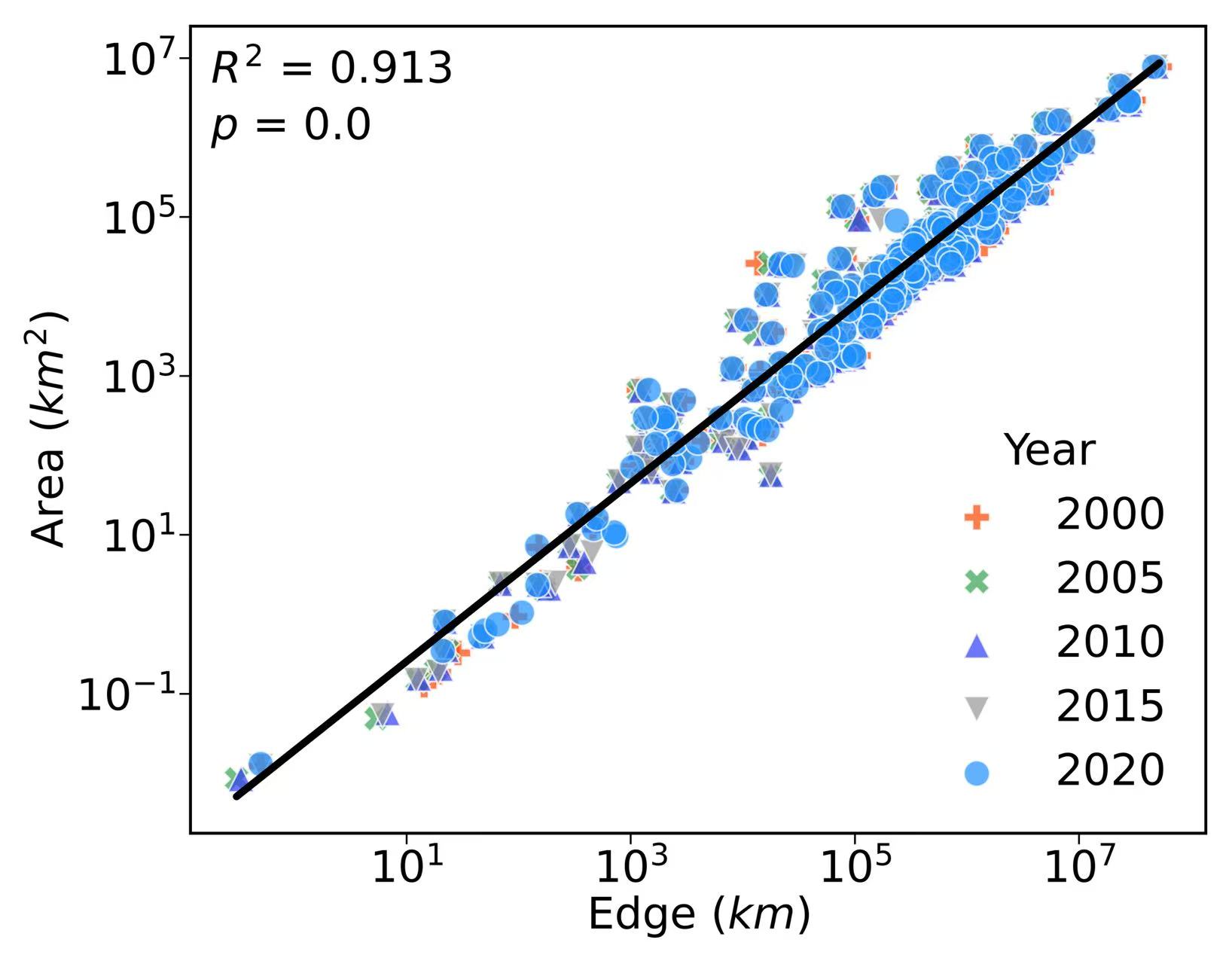
4. Forest edge and areas relationships
import matplotlib.pyplot as plt
import numpy as np
import pandas as pd
import warnings
from scipy import stats
warnings.filterwarnings('ignore')
def rsquared(x, y):
"""Return the metriscs coefficient of determination (R2)
Parameters:
-----------
x (numpy array or list): Predicted variables
y (numpy array or list): Observed variables
"""
slope, intercept, r_value, p_value, std_err = stats.linregress(x, y)
a = r_value**2
return a
#*************************
file_name = "/scratch/fji7/Forest_edge_mapping_2024_11_14/1_data/Country_Forest_Area_Edge.csv"
df = pd.read_csv(file_name)
df.dropna(inplace = True)
x1, x2, x3, x4, x5 = df["Total Forest Edge Length 2000 (KM)"],df["Total Forest Edge Length 2005 (KM)"],df["Total Forest Edge Length 2010 (KM)"],df["Total Forest Edge Length 2015 (KM)"],df["Total Forest Edge Length 2020 (KM)"]
y1, y2, y3, y4, y5 = df["Total Forest Area 2000 (KM2)"],df["Total Forest Area 2005 (KM2)"],df["Total Forest Area 2010 (KM2)"],df["Total Forest Area 2015 (KM2)"],df["Total Forest Area 2020 (KM2)"]
fig,ax = plt.subplots(figsize = (5,4))
config = {"font.family":'Helvetica'}
plt.subplots_adjust(hspace =0.2,wspace =0.2)
plt.rcParams.update(config)
x = [x1, x2, x3, x4, x5]
y = [y1, y2, y3, y4, y5]
colors = ["orangered", "#35a153","#303cf9", "#979797", "dodgerblue"]
markers = ["P", "X", "^", "v", "o"]
years = ["2000", "2005", "2010", "2015", "2020"]
a_total = []
b_total = []
for idx in range(5):
a,b = x[idx], y[idx]
a_total.extend(a)
b_total.extend(b)
ax.scatter(a,b,color=colors[idx], label=years[idx], alpha=0.7, edgecolors='w', linewidth=0.5, marker = markers[idx],s = 50)
final = pd.DataFrame([a_total,b_total]).T
final.columns = ["edge","area"]
final = final[(final['edge'] > 0) & (final['area'] > 0)]
coeffs = np.polyfit(np.log(final['edge']), np.log(final['area']), 1)
ax.plot(final['edge'], np.exp(coeffs[1]) * final['edge'] ** coeffs[0], color='k', linestyle='-', linewidth=2)
R2 = rsquared(final['edge'], final['area'])
_, p_value = stats.ttest_ind(final['edge'], final['area'])
ax.text(0.02, 0.93, f"$R^2$ = {round(R2,3)}", transform=ax.transAxes, color='k', fontsize=12)
ax.text(0.02, 0.86, f"$p$ = {round(p_value,5)}", transform=ax.transAxes, color='k', fontsize=12)
ax.set_xlabel('Edge ($km$)',fontsize=12,labelpad = 1)
ax.set_ylabel('Area ($km^2$)',fontsize=12,labelpad = 1)
ax.legend(title='Year',title_fontsize='large', scatterpoints=1, loc = 'lower right',fontsize=12,facecolor= 'none',edgecolor = 'none')
ax.tick_params(axis='both',which='major',labelsize=12,direction='out',length=3,width=0.5,pad=1.3,labelleft = True, labelbottom = True,
bottom=True,left=True,top=False,right=False)
ax.set_xscale('log')
ax.set_yscale('log')
plt.savefig('/scratch/fji7/Forest_edge_mapping_2024_11_14/2_exported_figures/Figure S5_forest edge_area relationships.png', dpi=1000, bbox_inches='tight')
-
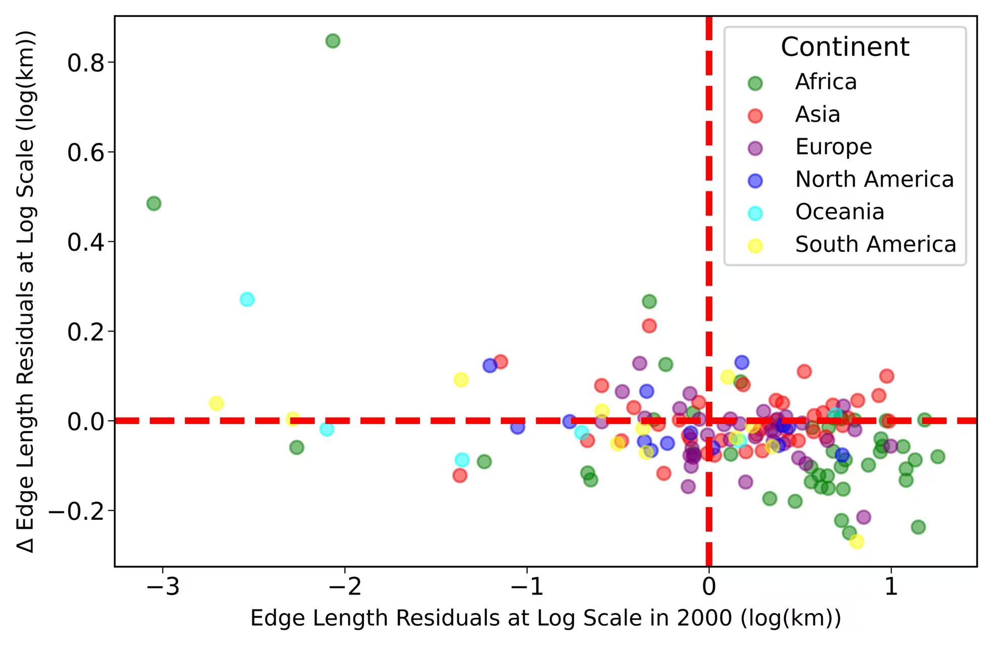
5. Forest landscape patterns
import matplotlib.pyplot as plt
import numpy as np
import pandas as pd
import warnings
from scipy import stats
import cartopy.io.shapereader as shpreader
warnings.filterwarnings('ignore')
def log_log_regression_model(log_x):
return intercept + slope * log_x
#*************************
file_name = "/scratch/fji7/Forest_edge_mapping_2024_11_14/1_data/Country_Forest_Area_Edge.csv"
df = pd.read_csv(file_name)
df.dropna(inplace = True)
# Calculating residuals for 2000
log_forest_area = np.log(df["Total Forest Area 2000 (KM2)"])
log_forest_edge = np.log(df["Total Forest Edge Length 2000 (KM)"])
slope, intercept, r_value, p_value, std_err = stats.linregress(log_forest_area, log_forest_edge)
log_estimated_forest_edge = log_log_regression_model(log_forest_area)
estimated_forest_edge = np.exp(log_estimated_forest_edge)
df['log_residuals2000'] = log_forest_edge - log_estimated_forest_edge
# Calculating residuals for 2020
log_forest_edge_2020 = np.log(df["Total Forest Edge Length 2020 (KM)"])
log_forest_area_2020 = np.log(df["Total Forest Area 2020 (KM2)"])
log_estimated_forest_edge_2020 = log_log_regression_model(log_forest_area_2020)
estimated_forest_edge_2020 = np.exp(log_estimated_forest_edge_2020)
df['log_residuals2020'] = log_forest_edge_2020 - log_estimated_forest_edge_2020
# Calculating delta residuals
df['delta_residuals'] = df['log_residuals2020'] - df['log_residuals2000']
# Output the results of the regression and the residuals
# slope, np.exp(intercept), r_value ** 2, p_value, df[['Country', 'log_residuals2000', 'log_residuals2020', 'delta_residuals']].head()
# Load the shapefile using Cartopy
shapefile = shpreader.natural_earth(resolution='110m', category='cultural', name='admin_0_countries')
reader = shpreader.Reader(shapefile)
# Create a dictionary mapping from country names to continents
country_to_continent = {country.attributes['NAME_LONG']: country.attributes['CONTINENT'] for country in reader.records()}
# Map each country in your dataframe to its continent
df['continent'] = df['Country'].map(country_to_continent)
# Define colors for each continent
colors = {
'Asia': 'red',
'Africa': 'green',
'North America': 'blue',
'South America': 'yellow',
'Europe': 'purple',
'Oceania': 'cyan',
'Antarctica': 'white'
}
# Map continents to colors in the dataframe
df['color'] = df['continent'].map(colors)
df.dropna(inplace = True)
fig,ax = plt.subplots(figsize = (7,4.5))
config = {"font.family":'Helvetica'}
plt.subplots_adjust(hspace =0.2,wspace =0.2)
plt.rcParams.update(config)
for continent, group in df.groupby('continent'):
ax.scatter(group['log_residuals2000'], group['delta_residuals'], color=group['color'], alpha=0.5, label=continent)
ax.axhline(0, color='red', linestyle='--', lw=3)
ax.axvline(0, color='red', linestyle='--', lw=3)
ax.set_xlabel('Edge Length Residuals at Log Scale in 2000 (log(km))' ,fontsize=10)
ax.set_ylabel('Δ Edge Length Residuals at Log Scale (log(km))',fontsize=10)
ax.tick_params(axis='both',which='major',labelsize=11,direction='out',length=3,width=0.5,pad=1.3,labelleft = True, labelbottom = True,
bottom=True,left=True,top=False,right=False)
ax.legend(title="Continent" ,title_fontsize='large', scatterpoints=1, loc = 'upper right',fontsize=10)
plt.savefig('/scratch/fji7/Forest_edge_mapping_2024_11_14/2_exported_figures/Figure S6_unequal development of forest landscape patterns.png', dpi=1000, bbox_inches='tight')